from fastai.tabular.all import *
from fastai.collab import *协同过滤教程
使用 fastai 库进行协同过滤。
本教程重点介绍如何快速构建一个 Learner 并在协同过滤任务上训练模型。
训练模型
在本教程中,我们将使用 Movielens 100k 数据集。我们可以轻松下载并使用以下函数解压它
path = untar_data(URLs.ML_100k)主表位于 u.data 中。由于它不是一个标准的 CSV 文件,我们在打开时需要指定一些信息:制表符分隔符、要保留的列及其名称。
ratings = pd.read_csv(path/'u.data', delimiter='\t', header=None,
                      usecols=(0,1,2), names=['user','movie','rating'])
ratings.head()| 用户 | 电影 | 评分 | |
|---|---|---|---|
| 0 | 196 | 242 | 3 |
| 1 | 186 | 302 | 3 |
| 2 | 22 | 377 | 1 |
| 3 | 244 | 51 | 2 |
| 4 | 166 | 346 | 1 |
电影 ID 不方便直观查看,因此我们加载了 u.item 表中对应的电影 ID 到标题的映射。
movies = pd.read_csv(path/'u.item',  delimiter='|', encoding='latin-1',
                     usecols=(0,1), names=('movie','title'), header=None)
movies.head()| 电影 | 标题 | |
|---|---|---|
| 0 | 1 | 玩具总动员 (1995) |
| 1 | 2 | 黄金眼 (1995) |
| 2 | 3 | 四个房间 (1995) |
| 3 | 4 | 矮子当道 (1995) |
| 4 | 5 | 跟屁虫 (1995) |
接下来我们将其合并到我们的评分表
ratings = ratings.merge(movies)
ratings.head()| 用户 | 电影 | 评分 | 标题 | |
|---|---|---|---|---|
| 0 | 196 | 242 | 3 | 柯利亚 (1996) |
| 1 | 63 | 242 | 3 | 柯利亚 (1996) |
| 2 | 226 | 242 | 5 | 柯利亚 (1996) |
| 3 | 154 | 242 | 3 | 柯利亚 (1996) |
| 4 | 306 | 242 | 5 | 柯利亚 (1996) |
然后我们可以从这张表构建一个 DataLoaders 对象。默认情况下,它将第一列作为用户,第二列作为项目(这里是我们的电影),第三列作为评分。在我们的例子中,我们需要改变 item_name 的值,以便使用标题而不是 ID。
dls = CollabDataLoaders.from_df(ratings, item_name='title', bs=64)在所有应用中,当数据组装到 DataLoaders 中后,你可以使用 show_batch 方法查看它。
dls.show_batch()| 用户 | 标题 | 评分 | |
|---|---|---|---|
| 0 | 181 | 替身 (1996) | 1 |
| 1 | 189 | 乌利的金子 (1997) | 3 |
| 2 | 6 | 洛城机密 (1997) | 4 |
| 3 | 849 | 网络 (1995) | 5 |
| 4 | 435 | 银翼杀手 (1982) | 4 |
| 5 | 718 | 我最好朋友的婚礼 (1997) | 4 |
| 6 | 279 | 我爱麻烦 (1994) | 2 |
| 7 | 561 | 发条橙 (1971) | 4 |
| 8 | 87 | 一条叫做旺达的鱼 (1988) | 5 |
| 9 | 774 | 乌鸦 (1994) | 3 |
fastai 可以使用 collab_learner 创建和训练协同过滤模型。
learn = collab_learner(dls, n_factors=50, y_range=(0, 5.5))它使用了一个简单的点积模型,包含 50 个潜在因子。要使用 1cycle 策略训练它,我们只需运行此命令
learn.fit_one_cycle(5, 5e-3, wd=0.1)| 周期 | 训练损失 | 验证损失 | 时间 |
|---|---|---|---|
| 0 | 0.967653 | 0.942309 | 00:10 |
| 1 | 0.843426 | 0.869254 | 00:10 |
| 2 | 0.733788 | 0.823143 | 00:10 |
| 3 | 0.593507 | 0.811050 | 00:10 |
| 4 | 0.480942 | 0.811475 | 00:10 |
这是针对流行的协同过滤系统 Librec 在同一数据集上的一些基准测试。它们显示基于 RMSE 的最佳结果为 0.91(向下滚动到 100k 数据集),这对应于 MSE 0.91**2 = 0.83。所以在不到一分钟的时间内,我们就获得了相当不错的结果!
解释
让我们分析一下之前模型的结果。我们将保留评分次数最多的 1000 部电影进行分析
g = ratings.groupby('title')['rating'].count()
top_movies = g.sort_values(ascending=False).index.values[:1000]
top_movies[:10]
array(['Star Wars (1977)', 'Contact (1997)', 'Fargo (1996)',
'Return of the Jedi (1983)', 'Liar Liar (1997)',
'English Patient, The (1996)', 'Scream (1996)', 'Toy Story (1995)',
'Air Force One (1997)', 'Independence Day (ID4) (1996)'],
dtype=object)电影偏差
我们的模型为每部电影学到了一个偏差(bias),这是一个独立于用户的独特数字,可以解释为电影的内在“价值”。我们可以使用以下命令从 top_movies 列表中获取每部电影的偏差。
movie_bias = learn.model.bias(top_movies, is_item=True)
movie_bias.shapetorch.Size([1000])让我们将这些偏差与平均评分进行比较
mean_ratings = ratings.groupby('title')['rating'].mean()
movie_ratings = [(b, i, mean_ratings.loc[i]) for i,b in zip(top_movies,movie_bias)]
现在让我们看看偏差最差的电影
item0 = lambda o:o[0]
sorted(movie_ratings, key=item0)[:15]
[(tensor(-0.3489),
'Children of the Corn: The Gathering (1996)',
1.3157894736842106),
(tensor(-0.3407), 'Leave It to Beaver (1997)', 1.8409090909090908),
(tensor(-0.3304), 'Cable Guy, The (1996)', 2.339622641509434),
(tensor(-0.2763),
'Lawnmower Man 2: Beyond Cyberspace (1996)',
1.7142857142857142),
(tensor(-0.2607), "McHale's Navy (1997)", 2.1884057971014492),
(tensor(-0.2572), 'Grease 2 (1982)', 2.0),
(tensor(-0.2482), 'Kansas City (1996)', 2.260869565217391),
(tensor(-0.2479), 'Crow: City of Angels, The (1996)', 1.9487179487179487),
(tensor(-0.2388), 'Free Willy 3: The Rescue (1997)', 1.7407407407407407),
(tensor(-0.2338), 'Keys to Tulsa (1997)', 2.24),
(tensor(-0.2305), 'Beautician and the Beast, The (1997)', 2.313953488372093),
(tensor(-0.2205), 'Escape from L.A. (1996)', 2.4615384615384617),
(tensor(-0.2192), 'Beverly Hills Ninja (1997)', 2.3125),
(tensor(-0.2179), 'Mortal Kombat: Annihilation (1997)', 1.9534883720930232),
(tensor(-0.2150), 'Thinner (1996)', 2.4489795918367347)]或者偏差最好的电影
sorted(movie_ratings, key=lambda o: o[0], reverse=True)[:15][(tensor(0.6052), 'As Good As It Gets (1997)', 4.196428571428571),
(tensor(0.5778), 'Titanic (1997)', 4.2457142857142856),
(tensor(0.5565), 'Shawshank Redemption, The (1994)', 4.445229681978798),
(tensor(0.5460), 'L.A. Confidential (1997)', 4.161616161616162),
(tensor(0.5264), 'Silence of the Lambs, The (1991)', 4.28974358974359),
(tensor(0.5125), 'Star Wars (1977)', 4.3584905660377355),
(tensor(0.4862), "Schindler's List (1993)", 4.466442953020135),
(tensor(0.4851), 'Rear Window (1954)', 4.3875598086124405),
(tensor(0.4671), 'Godfather, The (1972)', 4.283292978208232),
(tensor(0.4668), 'Apt Pupil (1998)', 4.1),
(tensor(0.4614), "One Flew Over the Cuckoo's Nest (1975)", 4.291666666666667),
(tensor(0.4606), 'Good Will Hunting (1997)', 4.262626262626263),
(tensor(0.4572), 'Contact (1997)', 3.8035363457760316),
(tensor(0.4529), 'Close Shave, A (1995)', 4.491071428571429),
(tensor(0.4410), 'Wrong Trousers, The (1993)', 4.466101694915254)]这确实存在很强的相关性!
电影权重
现在让我们尝试分析模型学到的潜在因子(latent factors)。我们可以像之前获取偏差(bias)一样,获取 top_movies 中每部电影的权重(weights)。
movie_w = learn.model.weight(top_movies, is_item=True)
movie_w.shape
torch.Size([1000, 50])让我们尝试使用 PCA 来降维,看看能否看出模型学到了什么。
movie_pca = movie_w.pca(3)
movie_pca.shape
torch.Size([1000, 3])fac0,fac1,fac2 = movie_pca.t()
movie_comp = [(f, i) for f,i in zip(fac0, top_movies)]这是在第一维上得分最高的电影
sorted(movie_comp, key=itemgetter(0), reverse=True)[:10][(tensor(1.1481), 'Casablanca (1942)'),
(tensor(1.0816), 'Chinatown (1974)'),
(tensor(1.0486), 'Lawrence of Arabia (1962)'),
(tensor(1.0459), 'Wrong Trousers, The (1993)'),
(tensor(1.0282), 'Secrets & Lies (1996)'),
(tensor(1.0245), '12 Angry Men (1957)'),
(tensor(1.0095), 'Some Folks Call It a Sling Blade (1993)'),
(tensor(0.9874), 'Close Shave, A (1995)'),
(tensor(0.9800), 'Wallace & Gromit: The Best of Aardman Animation (1996)'),
(tensor(0.9791), 'Citizen Kane (1941)')]以及得分最低的电影
sorted(movie_comp, key=itemgetter(0))[:10][(tensor(-1.2520), 'Home Alone 3 (1997)'),
(tensor(-1.2118), 'Jungle2Jungle (1997)'),
(tensor(-1.1282), 'Stupids, The (1996)'),
(tensor(-1.1229), 'Free Willy 3: The Rescue (1997)'),
(tensor(-1.1161), 'Leave It to Beaver (1997)'),
(tensor(-1.0821), 'Children of the Corn: The Gathering (1996)'),
(tensor(-1.0703), "McHale's Navy (1997)"),
(tensor(-1.0695), 'Bio-Dome (1996)'),
(tensor(-1.0652), 'Batman & Robin (1997)'),
(tensor(-1.0627), 'Cowboy Way, The (1994)')]第二维也是一样
movie_comp = [(f, i) for f,i in zip(fac1, top_movies)]sorted(movie_comp, key=itemgetter(0), reverse=True)[:10][(tensor(1.1196), 'Braveheart (1995)'),
(tensor(1.0969), 'Raiders of the Lost Ark (1981)'),
(tensor(1.0365), 'Independence Day (ID4) (1996)'),
(tensor(0.9631), 'Titanic (1997)'),
(tensor(0.9450), 'American President, The (1995)'),
(tensor(0.8893), 'Forrest Gump (1994)'),
(tensor(0.8757), 'Hunt for Red October, The (1990)'),
(tensor(0.8638), 'Pretty Woman (1990)'),
(tensor(0.8019), 'Miracle on 34th Street (1994)'),
(tensor(0.7956), 'True Lies (1994)')]sorted(movie_comp, key=itemgetter(0))[:10][(tensor(-0.9231), 'Ready to Wear (Pret-A-Porter) (1994)'),
(tensor(-0.8948), 'Dead Man (1995)'),
(tensor(-0.8816), 'Clockwork Orange, A (1971)'),
(tensor(-0.8697), 'Three Colors: Blue (1993)'),
(tensor(-0.8425), 'Beavis and Butt-head Do America (1996)'),
(tensor(-0.8047), 'Cable Guy, The (1996)'),
(tensor(-0.7832), 'Nosferatu (Nosferatu, eine Symphonie des Grauens) (1922)'),
(tensor(-0.7662), 'Exotica (1994)'),
(tensor(-0.7546), 'Spice World (1997)'),
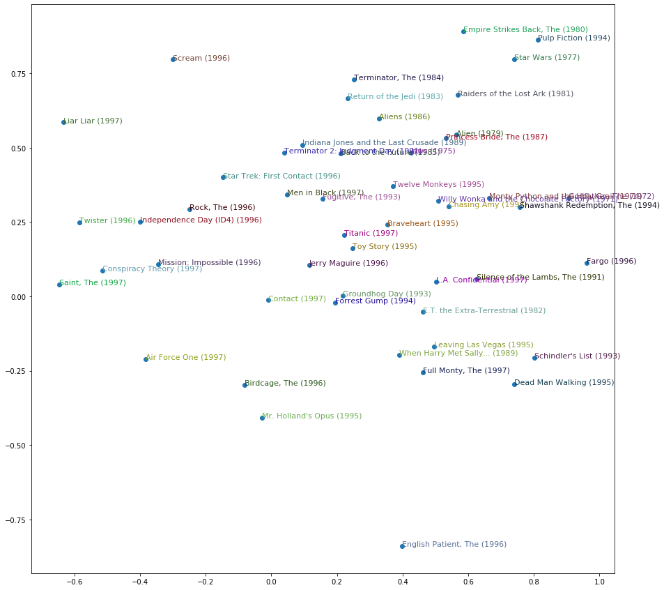
(tensor(-0.7491), 'Heavenly Creatures (1994)')]我们甚至可以根据电影在这些维度上的得分来绘制它们。
idxs = np.random.choice(len(top_movies), 50, replace=False)
idxs = list(range(50))
X = fac0[idxs]
Y = fac2[idxs]
plt.figure(figsize=(15,15))
plt.scatter(X, Y)
for i, x, y in zip(top_movies[idxs], X, Y):
    plt.text(x,y,i, color=np.random.rand(3)*0.7, fontsize=11)
plt.show()