超参数调度

用于调度任何超参数的回调函数和辅助函数

from fastai.test_utils import *

退火

---

源码

退火函数 (annealer)

 annealer (f)

使 f 返回其部分应用结果的装饰器。

这是我们将用于所有调度函数的装饰器，因为它将接受 (start, end, pos) 的函数转换为接受 (start, end) 并返回一个依赖于 pos 的函数。

---

源码

指数调度 (sched_exp)

 sched_exp (start, end, pos)

---

源码

常数调度 (sched_no)

 sched_no (start, end, pos)

---

源码

余弦调度 (sched_cos)

 sched_cos (start, end, pos)

---

源码

线性调度 (sched_lin)

 sched_lin (start, end, pos)

annealings = "NO LINEAR COS EXP".split()
p = torch.linspace(0.,1,100)
fns = [SchedNo, SchedLin, SchedCos, SchedExp]

for fn, t in zip(fns, annealings):
    plt.plot(p, [fn(2, 1e-2)(o) for o in p], label=t)
f = SchedPoly(2,1e-2,0.5)
plt.plot(p, [f(o) for o in p], label="POLY(0.5)")
plt.legend();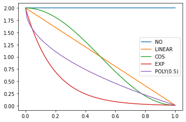

---

源码

SchedLin

 SchedLin (start, end)

从 start 到 end 的线性调度函数

sched = SchedLin(0, 2)
test_eq(L(map(sched, [0., 0.25, 0.5, 0.75, 1.])), [0., 0.5, 1., 1.5, 2.])

---

源码

SchedCos

 SchedCos (start, end)

从 start 到 end 的余弦调度函数

sched = SchedCos(0, 2)
test_close(L(map(sched, [0., 0.25, 0.5, 0.75, 1.])), [0., 0.29289, 1., 1.70711, 2.])

---

源码

SchedNo

 SchedNo (start, end)

具有 start 值的常数调度函数

sched = SchedNo(0, 2)
test_close(L(map(sched, [0., 0.25, 0.5, 0.75, 1.])), [0., 0., 0., 0., 0.])

---

源码

SchedExp

 SchedExp (start, end)

从 start 到 end 的指数调度函数

sched = SchedExp(1, 2)
test_close(L(map(sched, [0., 0.25, 0.5, 0.75, 1.])), [1., 1.18921, 1.41421, 1.68179, 2.])

---

源码

SchedPoly

 SchedPoly (start, end, power)

从 start 到 end 的多项式调度函数（power 次）

sched = SchedPoly(0, 2, 2)
test_close(L(map(sched, [0., 0.25, 0.5, 0.75, 1.])), [0., 0.125, 0.5, 1.125, 2.])

p = torch.linspace(0.,1,100)

pows = [0.5,1.,2.]
for e in pows:
    f = SchedPoly(2, 0, e)
    plt.plot(p, [f(o) for o in p], label=f'power {e}')
plt.legend();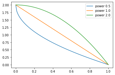

---

源码

组合调度 (combine_scheds)

 combine_scheds (pcts, scheds)

根据 pcts 将 scheds 组合成一个函数

pcts 必须是加起来等于 1 的正数列表，并且与 scheds 长度相同。生成的函数将从 0 到 pcts[0] 使用 scheds[0]，然后从 pcts[0] 到 pcts[0]+pcts[1] 使用 scheds[1]，依此类推。

p = torch.linspace(0.,1,100)
f = combine_scheds([0.3,0.7], [SchedCos(0.3,0.6), SchedCos(0.6,0.2)])
plt.plot(p, [f(o) for o in p]);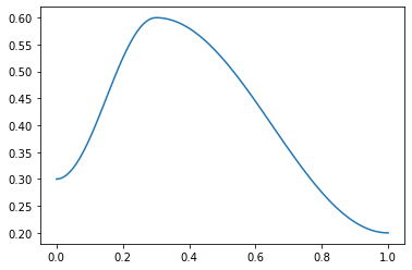

p = torch.linspace(0.,1,100)
f = combine_scheds([0.3,0.2,0.5], [SchedLin(0.,1.), SchedNo(1.,1.), SchedCos(1., 0.)])
plt.plot(p, [f(o) for o in p]);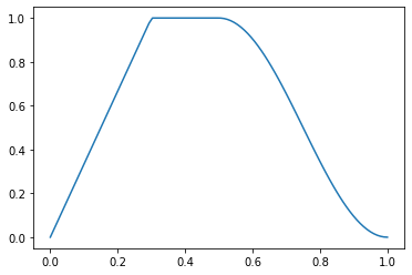

---

源码

组合余弦调度 (combined_cos)

 combined_cos (pct, start, middle, end)

返回一个从 start→middle 和 middle→end 进行余弦退火的调度器

这是针对 1cycle 策略的一个有用辅助函数。pct 用于 start 到 middle 部分，1-pct 用于 middle 到 end 部分。支持浮点数或浮点数集合。例如

f = combined_cos(0.25,0.5,1.,0.)
plt.plot(p, [f(o) for o in p]);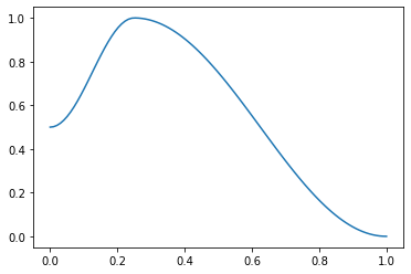

---

源码

参数调度器 (ParamScheduler)

 ParamScheduler (scheds)

根据 scheds 调度超参数

scheds 是一个字典，其中每个你想调度的超参数对应一个键，值可以是单个调度器或调度器列表（后一种情况下，列表长度必须与优化器的参数组数量相同）。

learn = synth_learner()
sched = {'lr': SchedLin(1e-3, 1e-2)}
learn.fit(1, cbs=ParamScheduler(sched))
n = len(learn.dls.train)
test_close(learn.recorder.hps['lr'], [1e-3 + (1e-2-1e-3) * i/n for i in range(n)])

epoch	训练损失 (train_loss)	验证损失 (valid_loss)	时间
0	11.929138	4.039281	00:00

---

源码

ParamScheduler.before_fit

 ParamScheduler.before_fit ()

初始化超参数容器

---

源码

ParamScheduler.before_batch

 ParamScheduler.before_batch ()

在优化器中设置适当的超参数

---

源码

ParamScheduler.after_batch

 ParamScheduler.after_batch ()

记录此批次的超参数

---

源码

ParamScheduler.after_fit

 ParamScheduler.after_fit ()

如果存在 recorder，将超参数保存到其中

---

源码

Learner.fit_one_cycle

 Learner.fit_one_cycle (n_epoch, lr_max=None, div=25.0,
                        div_final=100000.0, pct_start=0.25, wd=None,
                        moms=None, cbs=None, reset_opt=False,
                        start_epoch=0)

使用 1cycle 策略训练 self.model 共 n_epoch 个周期。

1cycle 策略由 Leslie N. Smith 等人在 Super-Convergence: Very Fast Training of Neural Networks Using Large Learning Rates 中提出。它使用余弦退火策略调度学习率，从 lr_max/div 到 lr_max，然后再到 lr_max/div_final（如果你想使用差异学习率，可以将数组传递给 lr_max），并根据 moms 中的值使用余弦退火调度动量。第一阶段占用训练的 pct_start。你可以选择性地传递额外的 cbs 和 reset_opt。

#Integration test: training a few epochs should make the model better
learn = synth_learner(lr=1e-2)
xb,yb = learn.dls.one_batch()
init_loss = learn.loss_func(learn.model(xb), yb)
learn.fit_one_cycle(2)
xb,yb = learn.dls.one_batch()
final_loss = learn.loss_func(learn.model(xb), yb)
assert final_loss < init_loss

epoch	训练损失 (train_loss)	验证损失 (valid_loss)	时间
0	19.444899	6.755066	00:00
1	9.919473	1.044571	00:00

#Scheduler test
lrs,moms = learn.recorder.hps['lr'],learn.recorder.hps['mom']
test_close(lrs,  [combined_cos(0.25,1e-2/25,1e-2,1e-7)(i/20) for i in range(20)])
test_close(moms, [combined_cos(0.25,0.95,0.85,0.95)(i/20) for i in range(20)])

---

源码

Recorder.plot_sched

 Recorder.plot_sched (keys=None, figsize=None)

learn = synth_learner()
learn.fit_one_cycle(2)

epoch	训练损失 (train_loss)	验证损失 (valid_loss)	时间
0	5.406837	5.305011	00:00
1	5.058437	4.899223	00:00

learn.recorder.plot_sched()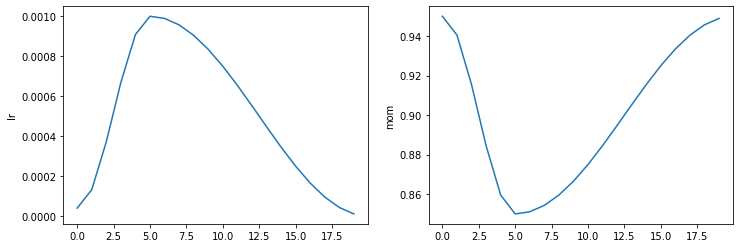

---

源码

Learner.fit_flat_cos

 Learner.fit_flat_cos (n_epoch, lr=None, div_final=100000.0,
                       pct_start=0.75, wd=None, cbs=None, reset_opt=False,
                       start_epoch=0)

在余弦退火之前，以固定的 lr 训练 self.model 共 n_epoch 个周期。

learn = synth_learner()
learn.fit_flat_cos(2)

epoch	训练损失 (train_loss)	验证损失 (valid_loss)	时间
0	10.588930	7.106113	00:00
1	8.943380	5.016665	00:00

learn.recorder.plot_sched()

---

源码

Learner.fit_sgdr

 Learner.fit_sgdr (n_cycles, cycle_len, lr_max=None, cycle_mult=2,
                   cbs=None, reset_opt=False, wd=None, start_epoch=0)

使用 SGDR 训练 self.model 共 n_cycles 个周期，每个周期长度为 cycle_len。

该调度策略由 Ilya Loshchilov 等人在 SGDR: Stochastic Gradient Descent with Warm Restarts 中提出。它包含 n_cycles 个周期，每个周期都是从 lr_max（默认为 Learner 的学习率）到 0 的余弦退火过程，其中第 i 个周期的长度为 cycle_len * cycle_mult**i（第一个周期长度为 cycle_len，然后我们在每个周期将长度乘以 cycle_mult）。你可以选择性地传递额外的 cbs 和 reset_opt。

learn = synth_learner()
with learn.no_logging(): learn.fit_sgdr(3, 1)
test_eq(learn.n_epoch, 7)
iters = [k * len(learn.dls.train) for k in [0,1,3,7]]
for i in range(3):
    n = iters[i+1]-iters[i]
    #The start of a cycle can be mixed with the 0 of the previous cycle with rounding errors, so we test at +1
    test_close(learn.recorder.lrs[iters[i]+1:iters[i+1]], [SchedCos(learn.lr, 0)(k/n) for k in range(1,n)])

learn.recorder.plot_sched()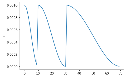

---

源码

Learner.fine_tune

 Learner.fine_tune (epochs, base_lr=0.002, freeze_epochs=1, lr_mult=100,
                    pct_start=0.3, div=5.0, lr_max=None,
                    div_final=100000.0, wd=None, moms=None, cbs=None,
                    reset_opt=False, start_epoch=0)

先使用 Learner.freeze 微调 freeze_epochs 个周期，然后使用 Learner.unfreeze 微调 epochs 个周期，使用差异学习率。

learn.fine_tune(1)

epoch	训练损失 (train_loss)	验证损失 (valid_loss)	时间
0	2.428970	1.740237	00:00

epoch	训练损失 (train_loss)	验证损失 (valid_loss)	时间
0	2.019952	1.616970	00:00

从检查点恢复训练

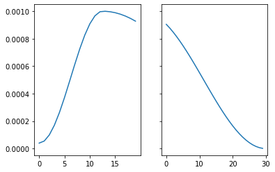
要启用从检查点恢复，请务必保存模型和优化器状态。这可以通过使用 SaveModelCallback 并设置 (with_opt=True) 来完成。如果训练中断，请使用与之前相同的参数定义 learn，从检查点加载模型，并将 start_epoch 传递给 fit 调用。训练将从 start_epoch 开始，并使用适当调度的 lr 继续进行。

with tempfile.TemporaryDirectory() as d:
    learn1 = synth_learner(path=d, cbs=SaveModelCallback(with_opt=True, fname="ckpt"))
    learn1.fit_one_cycle(5, cbs=InterruptCallback(2))
    
    learn2 = synth_learner(path=d)
    learn2 = learn2.load("ckpt")
    learn2.fit_one_cycle(5, start_epoch=2)
    
    fig, axs = plt.subplots(1,2, sharey=True)
    axs[0].plot(learn1.recorder.lrs)
    axs[1].plot(learn2.recorder.lrs)

epoch	训练损失 (train_loss)	验证损失 (valid_loss)	时间
0	18.930223	14.100439	00:00
1	17.092665	10.603369	00:00

Better model found at epoch 0 with valid_loss value: 14.100439071655273.
Better model found at epoch 1 with valid_loss value: 10.603368759155273.

epoch	训练损失 (train_loss)	验证损失 (valid_loss)	时间
0	00:00
1	00:00
2	11.456764	10.057186	00:00
3	10.287196	8.694046	00:00
4	9.585465	8.422710	00:00

---

源码

LRFinder

 LRFinder (start_lr=1e-07, end_lr=10, num_it=100, stop_div=True)

使用指数增长的学习率进行训练

from fastai.vision.all import *

set_seed(99, True)
path = untar_data(URLs.PETS)/'images'

image_files = get_image_files(path)
if sys.platform == "win32" and IN_NOTEBOOK:
    image_files = random.choices(image_files, k=int(len(image_files)/8))
    print("Randomly select 1/8 files in NOTEBOOK on Windows to save time")

# pickle can't serializer lamda function.
def _label_func(x):
    return x[0].isupper()

dls = ImageDataLoaders.from_name_func(
    path, image_files, valid_pct=0.2,
    label_func=_label_func, item_tfms=Resize(224))

learn = vision_learner(dls, resnet18)
learn.fit(1)
learn.opt.state_dict()['state'][1]['grad_avg']

epoch	训练损失 (train_loss)	验证损失 (valid_loss)	时间
0	0.086690	0.016682	00:33

tensor([-5.8191e-04, -2.2443e-03,  0.0000e+00, -1.2517e-03,  0.0000e+00,
        -1.4744e-03, -3.6433e-04,  0.0000e+00,  9.3745e-03,  0.0000e+00,
         5.1993e-03, -1.5093e-02, -4.0410e-03,  0.0000e+00,  7.1963e-03,
        -6.6033e-03, -3.3354e-03, -2.9191e-03, -1.5054e-03, -1.3179e-03,
         8.7333e-03, -1.1155e-02, -9.6656e-04,  1.6653e-02,  9.5839e-04,
         8.4995e-03, -2.8187e-02,  3.1579e-03, -9.3051e-04, -2.3887e-03,
        -7.3557e-04, -1.4501e-02, -6.2110e-03,  1.9949e-03, -7.0233e-03,
         1.2792e-02,  0.0000e+00,  1.0687e-03,  0.0000e+00, -4.2413e-04,
         2.9628e-03,  7.2686e-03, -9.7241e-03, -4.9941e-04,  1.7408e-02,
        -9.2441e-03, -9.7731e-03, -9.9393e-03,  0.0000e+00, -2.1448e-03,
         2.7660e-03, -3.1110e-03,  5.9454e-05, -1.4412e-03, -6.1454e-04,
        -1.6537e-03,  1.7001e-02,  1.4041e-02, -6.2878e-03,  2.0800e-02,
        -1.2900e-02, -1.2626e-02, -2.6591e-03,  3.9685e-03], device='cuda:0')

with tempfile.TemporaryDirectory() as d:
    learn = synth_learner(path=Path(d))
    init_a,init_b = learn.model.a,learn.model.b
    with learn.no_logging(): learn.fit(20, cbs=LRFinder(num_it=100))
    assert len(learn.recorder.lrs) <= 100
    test_eq(len(learn.recorder.lrs), len(learn.recorder.losses))
    #Check stop if diverge
    if len(learn.recorder.lrs) < 100: assert learn.recorder.losses[-1] > 4 * min(learn.recorder.losses)
    #Test schedule
    test_eq(learn.recorder.lrs, [SchedExp(1e-7, 10)(i/100) for i in range_of(learn.recorder.lrs)])
    #No validation data
    test_eq([len(v) for v in learn.recorder.values], [1 for _ in range_of(learn.recorder.values)])
    #Model loaded back properly
    test_eq(learn.model.a, init_a)
    test_eq(learn.model.b, init_b)
    test_eq(learn.opt.state_dict()['state'], [{}, {}])

---

源码

LRFinder.before_fit

 LRFinder.before_fit ()

初始化超参数容器并保存模型

---

源码

LRFinder.before_batch

 LRFinder.before_batch ()

在优化器中设置适当的超参数

---

源码

LRFinder.after_batch

 LRFinder.after_batch ()

记录此批次的超参数并可能停止训练

---

源码

LRFinder.before_validate

 LRFinder.before_validate ()

跳过训练的验证部分

建议方法

有几种自动建议学习率的方法，正如我们将看到的，这些方法可以进一步传递给 lr_find。目前支持四种方法，但是要编写自己的方法，它应该看起来像一个函数，可以接受 LRFinder 返回的 lrs、losses 以及 num_it。你的函数应该返回一个可以绘制的 x,y 坐标，如下所示

def myfunc(lrs:list, losses:list, num_it:int) -> tuple(float, tuple(float,int)):
    ...
    return suggestion, (suggestion,loss_idx)

如果还有其他需要传入的参数，你应该将 func 作为 partial 传入并自行指定，例如

def myfunc(lrs:list, losses:list, num_it:int, pct_reduction:float) -> tuple(float, tuple(float,int)):
    ...
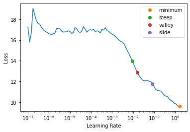
    return suggestion, (suggestion,loss_idx)

f = partial(myfunc, pct_reduction=.2)

---

源码

valley (波谷)

 valley (lrs:list, losses:list, num_it:int)

从最长的波谷建议一个学习率并返回其索引

valley 算法由 ESRI 开发，取 LR 曲线最长波谷约 2/3 处的最陡斜率对应的学习率，也是 Learner.lr_find 的默认方法。

---

源码

slide (滑动)

 slide (lrs:list, losses:list, num_it:int, lr_diff:int=15,
        thresh:float=0.005, adjust_value:float=1.0)

根据区间滑动规则建议一个学习率并返回其索引

slide 规则是 Andrew Chang 在 Novetta 开发的一种算法，详情见此处。

---

源码

minimum (最小值)

 minimum (lrs:list, losses:list, num_it:int)

建议一个在发散前最小值十分之一处的学习率并返回其索引

---

源码

steep (最陡)

 steep (lrs:list, losses:list, num_it:int)

建议一个斜率最陡峭时的学习率并返回其索引

---

源码

Recorder.plot_lr_find

 Recorder.plot_lr_find (skip_end=5, return_fig=True, suggestions=None,
                        nms=None, **kwargs)

绘制 LR Finder 测试结果（如果您之前没有运行 learn.lr_find() 则无法工作）

---

源码

Learner.lr_find

 Learner.lr_find (start_lr=1e-07, end_lr=10, num_it=100, stop_div=True,
                  show_plot=True, suggest_funcs=<function valley>)

启动模拟训练以寻找合适的学习率，并根据 suggest_funcs 返回命名元组形式的建议结果

LR Finder 最早由 Leslie N. Smith 在 Cyclical Learning Rates for Training Neural Networks 中提出，它通过从 start_lr 到 end_lr 的指数增长学习率训练模型 num_it 次迭代，并在发生发散时停止（除非设置 stop_div=False），然后以对数刻度绘制损失与学习率的关系图。

可以将多种学习率建议算法传递给该函数，默认情况下我们使用 valley 方法。

with tempfile.TemporaryDirectory() as d:
    learn = synth_learner(path=Path(d))
    weights_pre_lr_find = L(learn.model.parameters())
    lr_min, lr_steep, lr_valley, lr_slide = learn.lr_find(suggest_funcs=(minimum, steep, valley, slide))
    weights_post_lr_find = L(learn.model.parameters())
test_eq(weights_pre_lr_find, weights_post_lr_find)
print(f"Minimum/10:\t{lr_min:.2e}\nSteepest point:\t{lr_steep:.2e}\nLongest valley:\t{lr_valley:.2e}\nSlide interval:\t{lr_slide:.2e}")

Minimum/10: 1.58e-01
Steepest point: 9.12e-03
Longest valley: 1.58e-02
Slide interval: 8.32e-02